Chapter 5 04-Basketball
5.1 Intro
This chapter explores NBA player performance using team total data from the 2024–2025 season. I create composite metrics for offense (PRA: points + rebounds + assists) and defense (STOCKS: steals + blocks), merge team-level conference information, and compare distributions across East vs. West. I use visualizations, point-biserial correlations, a correlation matrix, and partial correlation to examine relationships between age and performance metrics.
5.2
load_team_data <- function(sheet_name, file_path = "NBA Team Total Data 2024-2025.xlsx") {
  df <- read_excel(file_path, sheet = sheet_name)

  df <- df %>%
    mutate(
      Team = sheet_name,
      Won_award = ifelse(is.na(Awards), 0, 1),
      PRA = PTS + TRB + AST,
      STOCKS = STL + BLK
    )

  return(df)
}


file_path <- "NBA Team Total Data 2024-2025.xlsx"


team_sheets <- excel_sheets(file_path)


all_teams_list <- lapply(team_sheets, load_team_data, file_path = file_path)


nba_data <- bind_rows(all_teams_list)


head(nba_data)
## # A tibble: 6 × 35
## Rk Player Age G GS MP FG FGA `FG%` `3P` `3PA` `3P%` `2P`
## <dbl> <chr> <dbl> <dbl> <dbl> <dbl> <dbl> <dbl> <dbl> <dbl> <dbl> <dbl> <dbl>
## 1 1 Jalen… 24 79 22 2031 246 620 0.397 122 362 0.337 124
## 2 2 Keon … 22 79 56 1925 303 779 0.389 126 401 0.314 177
## 3 3 Nic C… 25 70 62 1882 320 568 0.563 5 21 0.238 315
## 4 4 Camer… 28 57 57 1800 355 747 0.475 159 408 0.39 196
## 5 5 Ziair… 23 63 45 1541 214 520 0.412 103 302 0.341 111
## 6 6 Tyres… 25 60 11 1315 189 465 0.406 99 282 0.351 90
## # ℹ 22 more variables: `2PA` <dbl>, `2P%` <dbl>, `eFG%` <dbl>, FT <dbl>,
## # FTA <dbl>, `FT%` <dbl>, ORB <dbl>, DRB <dbl>, TRB <dbl>, AST <dbl>,
## # STL <dbl>, BLK <dbl>, TOV <dbl>, PF <dbl>, PTS <dbl>, `Trp-Dbl` <dbl>,
## # Awards <chr>, Team <chr>, Won_award <dbl>, PRA <dbl>, STOCKS <dbl>,
## # Pos <chr>5.3
conference_lookup <- read_excel("Team Conferences.xlsx")


nba_data <- nba_data %>%
  left_join(conference_lookup, by = "Team") %>%
  mutate(Conference_binary = ifelse(Conference == "East", 1, 0))

head(nba_data)
## # A tibble: 6 × 37
## Rk Player Age G GS MP FG FGA `FG%` `3P` `3PA` `3P%` `2P`
## <dbl> <chr> <dbl> <dbl> <dbl> <dbl> <dbl> <dbl> <dbl> <dbl> <dbl> <dbl> <dbl>
## 1 1 Jalen… 24 79 22 2031 246 620 0.397 122 362 0.337 124
## 2 2 Keon … 22 79 56 1925 303 779 0.389 126 401 0.314 177
## 3 3 Nic C… 25 70 62 1882 320 568 0.563 5 21 0.238 315
## 4 4 Camer… 28 57 57 1800 355 747 0.475 159 408 0.39 196
## 5 5 Ziair… 23 63 45 1541 214 520 0.412 103 302 0.341 111
## 6 6 Tyres… 25 60 11 1315 189 465 0.406 99 282 0.351 90
## # ℹ 24 more variables: `2PA` <dbl>, `2P%` <dbl>, `eFG%` <dbl>, FT <dbl>,
## # FTA <dbl>, `FT%` <dbl>, ORB <dbl>, DRB <dbl>, TRB <dbl>, AST <dbl>,
## # STL <dbl>, BLK <dbl>, TOV <dbl>, PF <dbl>, PTS <dbl>, `Trp-Dbl` <dbl>,
## # Awards <chr>, Team <chr>, Won_award <dbl>, PRA <dbl>, STOCKS <dbl>,
## # Pos <chr>, Conference <chr>, Conference_binary <dbl>ggplot(nba_data, aes(x = PRA, y = STOCKS, color = factor(Conference_binary))) +
geom_point(size = 3, alpha = 0.7) +
labs(color = "Conference (1=East, 0=West)",
x = "PRA (Points + Rebounds + Assists)",
y = "STOCKS (Steals + Blocks)",
title = "Offensive vs Defensive Performance by Conference") +
theme_minimal()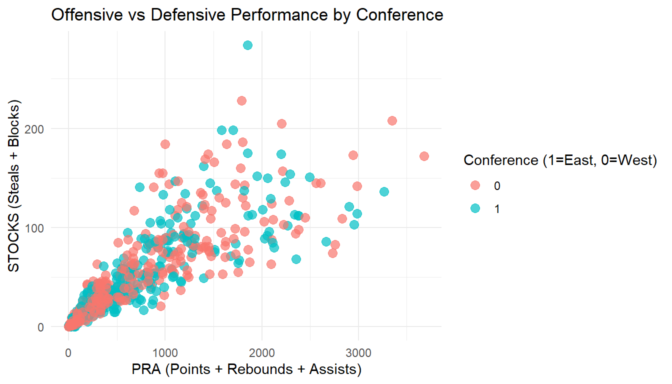
Figure 5.1: Scatterplot of offensive output (PRA) versus defensive output (STOCKS), colored by conference (East vs West). This visual compares overall player performance patterns by conference.
ggplot(nba_data, aes(x = PRA, fill = factor(Conference_binary))) +
  geom_histogram(position = "dodge", bins = 15, alpha = 0.7) +
  labs(fill = "Conference (1=East, 0=West)",
       x = "PRA",
       y = "Number of Players",
       title = "Distribution of PRA by Conference") +
  theme_minimal()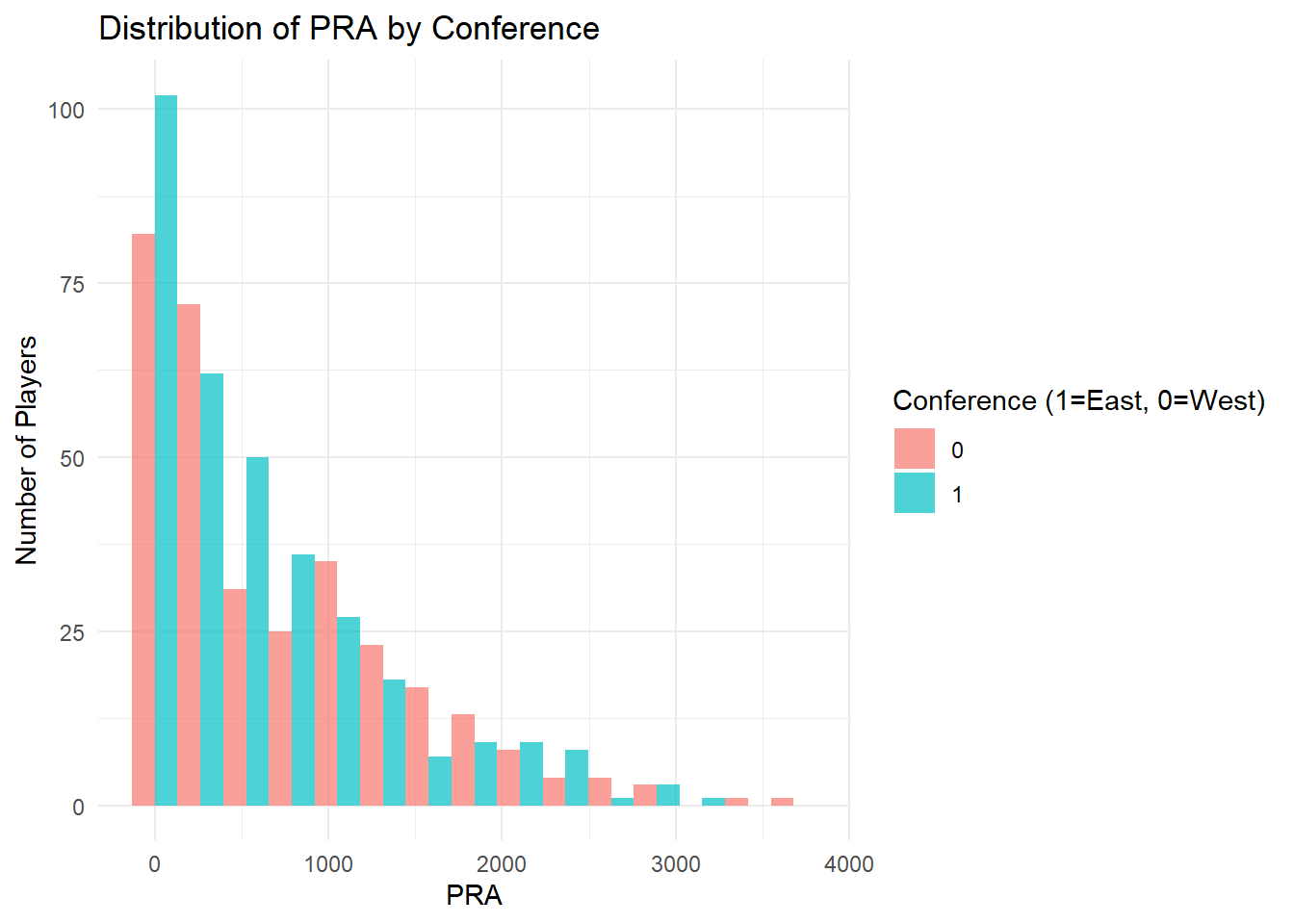
Figure 5.2: Distribution of PRA by Conference
cor_pra <- cor.test(nba_data$Conference_binary, nba_data$PRA)
cor_stocks <- cor.test(nba_data$Conference_binary, nba_data$STOCKS)

cor_pra
##
## Pearson's product-moment correlation
##
## data: nba_data$Conference_binary and nba_data$PRA
## t = -1.8195, df = 650, p-value = 0.0693
## alternative hypothesis: true correlation is not equal to 0
## 95 percent confidence interval:
## -0.147164250 0.005629906
## sample estimates:
## cor
## -0.07118475##
## Pearson's product-moment correlation
##
## data: nba_data$Conference_binary and nba_data$STOCKS
## t = -2.094, df = 650, p-value = 0.03665
## alternative hypothesis: true correlation is not equal to 0
## 95 percent confidence interval:
## -0.157650363 -0.005105577
## sample estimates:
## cor
## -0.08185737cor_matrix <- nba_data %>%
dplyr::select(Age, PRA, STOCKS) %>%
cor(use = "pairwise.complete.obs")
ggcorrplot(cor_matrix, lab = TRUE, title = "Correlation Matrix: Age, PRA, STOCKS")## Warning: `aes_string()` was deprecated in ggplot2 3.0.0.
## ℹ Please use tidy evaluation idioms with `aes()`.
## ℹ See also `vignette("ggplot2-in-packages")` for more information.
## ℹ The deprecated feature was likely used in the ggcorrplot package.
## Please report the issue at <https://github.com/kassambara/ggcorrplot/issues>.
## This warning is displayed once every 8 hours.
## Call `lifecycle::last_lifecycle_warnings()` to see where this warning was
## generated.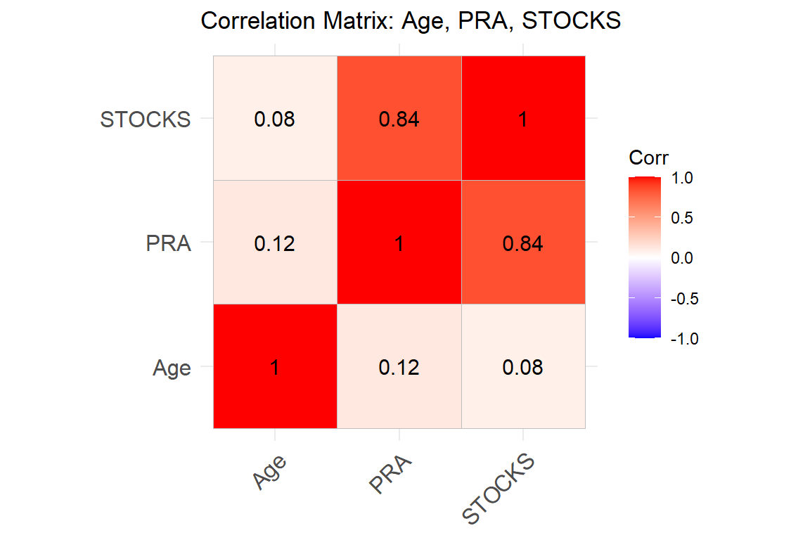
Figure 5.3: Correlation matrix for Age, PRA, and STOCKS. Values summarize the direction and strength of associations among these variables.
##    estimate       p.value statistic   n gp  Method
## 1 0.8395996 3.657553e-174  39.37587 652  1 pearson
5.4
Point-biserial correlations were used to test whether conference membership relates to PRA and STOCKS. A partial correlation tested the association between PRA and STOCKS while controlling for age.