Chapter 4 03-Sleep

4.1 Chapter introduction

This chapter analyzes a dataset examining whether different exercise routines are associated with improvements in sleep. Using data cleaning, merging, descriptive statistics, visualizations, t-tests, and one-way ANOVA with post-hoc comparisons, I evaluate changes in sleep duration (post–pre) and sleep efficiency across exercise groups. This provides practice working with real-world messy inputs, reproducible workflows, and interpreting statistical results.

file_path <- "C:/Users/laura/OneDrive/Desktop/real_bookdown/midterm_sleep_exercise.xlsx"
participant_info <- read_xlsx(file_path, sheet = "participant_info_midterm")
sleep_data       <- read_xlsx(file_path, sheet = "sleep_data_midterm")

participant_info <- clean_names(participant_info)
sleep_data       <- clean_names(sleep_data)

head(participant_info)

## # A tibble: 6 × 4
##   id    exercise_group sex      age
##   <chr> <chr>          <chr>  <dbl>
## 1 P001  NONE           Male      35
## 2 P002  Nonee          Malee     57
## 3 P003  None           Female    26
## 4 P004  None           Female    29
## 5 P005  None           Male      33
## 6 P006  None           Female    33

head(sleep_data)

## # A tibble: 6 × 4
##   id    pre_sleep post_sleep sleep_efficiency
##   <chr> <chr>          <dbl>            <dbl>
## 1 P001  zzz-5.8          4.7             81.6
## 2 P002  Sleep-6.6        7.4             75.7
## 3 P003  <NA>             6.2             82.9
## 4 P004  SLEEP-7.2        7.3             83.6
## 5 P005  score-7.4        7.4             83.5
## 6 P006  Sleep-6.6        7.1             88.5

4.2

merged_data <- left_join(participant_info, sleep_data, by = "id") %>%
  mutate(
    sex = case_when(
      tolower(sex) %in% c("female","fem","f","femalee") ~ "Female",
      tolower(sex) %in% c("male","mal","m","malee") ~ "Male",
      TRUE ~ NA_character_
    ),
    exercise_group = case_when(
      str_detect(tolower(exercise_group), "c\\+w|cw") ~ "C+W",
      str_detect(tolower(exercise_group), "cardio") ~ "Cardio",
      str_detect(tolower(exercise_group), "weights|weight") ~ "Weights",
      str_detect(tolower(exercise_group), "none") ~ "None",
      TRUE ~ exercise_group
    ),
    age = as.numeric(age),
    pre_sleep = as.numeric(str_extract(pre_sleep, "\\d+\\.\\d+")),
    post_sleep = as.numeric(post_sleep),
    sleep_difference = post_sleep - pre_sleep,
    agegroup2 = case_when(
      age < 40 ~ "<40",
      age >= 40 ~ ">=40",
      TRUE ~ NA_character_
    )
  ) %>%
  filter(!is.na(sleep_difference))

knitr::kable(table(merged_data$exercise_group),
             caption = "Number of participants in each exercise group.")

Table 4.1: Number of participants in each exercise group.
Var1	Freq
C+W	3
Cardio	34
N	2
None	15
Weights	19

knitr::kable(table(merged_data$sex),
             caption = "Number of participants by sex.")

Table 4.1: Number of participants by sex.
Var1	Freq
Female	40
Male	33

knitr::kable(table(merged_data$agegroup2),
             caption = "Number of participants by age group (<40 vs ≥40).")

Table 4.1: Number of participants by age group (<40 vs ≥40).
Var1	Freq
<40	57
>=40	16

4.3

summary(merged_data$sleep_difference)

##    Min. 1st Qu.  Median    Mean 3rd Qu.    Max. 
## -1.1000  0.3000  0.8000  0.6822  1.1000  2.0000

overall_summary <- merged_data %>%
summarise(
mean_sleep_diff = mean(sleep_difference),
sd_sleep_diff   = sd(sleep_difference),
min_sleep_diff  = min(sleep_difference),
max_sleep_diff  = max(sleep_difference),
mean_sleep_eff  = mean(sleep_efficiency),
sd_sleep_eff    = sd(sleep_efficiency),
min_sleep_eff   = min(sleep_efficiency),
max_sleep_eff   = max(sleep_efficiency)
)
knitr::kable(overall_summary, digits = 2,
             caption = "Overall descriptive statistics for sleep difference (post–pre) and sleep efficiency.")

Table 4.2: Overall descriptive statistics for sleep difference (post–pre) and sleep efficiency.
mean_sleep_diff	sd_sleep_diff	min_sleep_diff	max_sleep_diff	mean_sleep_eff	sd_sleep_eff	min_sleep_eff	max_sleep_eff
0.68	0.63	-1.1	2	84.16	5.98	71.7	101.5

group_summary <- merged_data %>%
group_by(exercise_group) %>%
summarise(
mean_sleep_diff = mean(sleep_difference),
sd_sleep_diff   = sd(sleep_difference),
mean_sleep_eff  = mean(sleep_efficiency),
sd_sleep_eff    = sd(sleep_efficiency),
n = n()
)
knitr::kable(group_summary, digits = 2,
             caption = "Descriptive statistics for sleep difference and sleep efficiency by exercise group.")

Table 4.2: Descriptive statistics for sleep difference and sleep efficiency by exercise group.
exercise_group	mean_sleep_diff	sd_sleep_diff	mean_sleep_eff	sd_sleep_eff	n
C+W	1.10	0.10	90.23	3.76	3
Cardio	0.97	0.44	86.56	5.94	34
N	0.30	0.85	81.30	0.28	2
None	0.09	0.64	81.37	6.10	15
Weights	0.61	0.60	81.43	3.92	19

4.4

ggplot(merged_data, aes(x = exercise_group, y = sleep_difference, fill = exercise_group)) +
  geom_boxplot() +
  labs(title = "Sleep Improvement by Exercise Group",
       x = "Exercise Group", y = "Sleep Difference (Post - Pre)") +
  theme_minimal() +
  theme(legend.position = "none")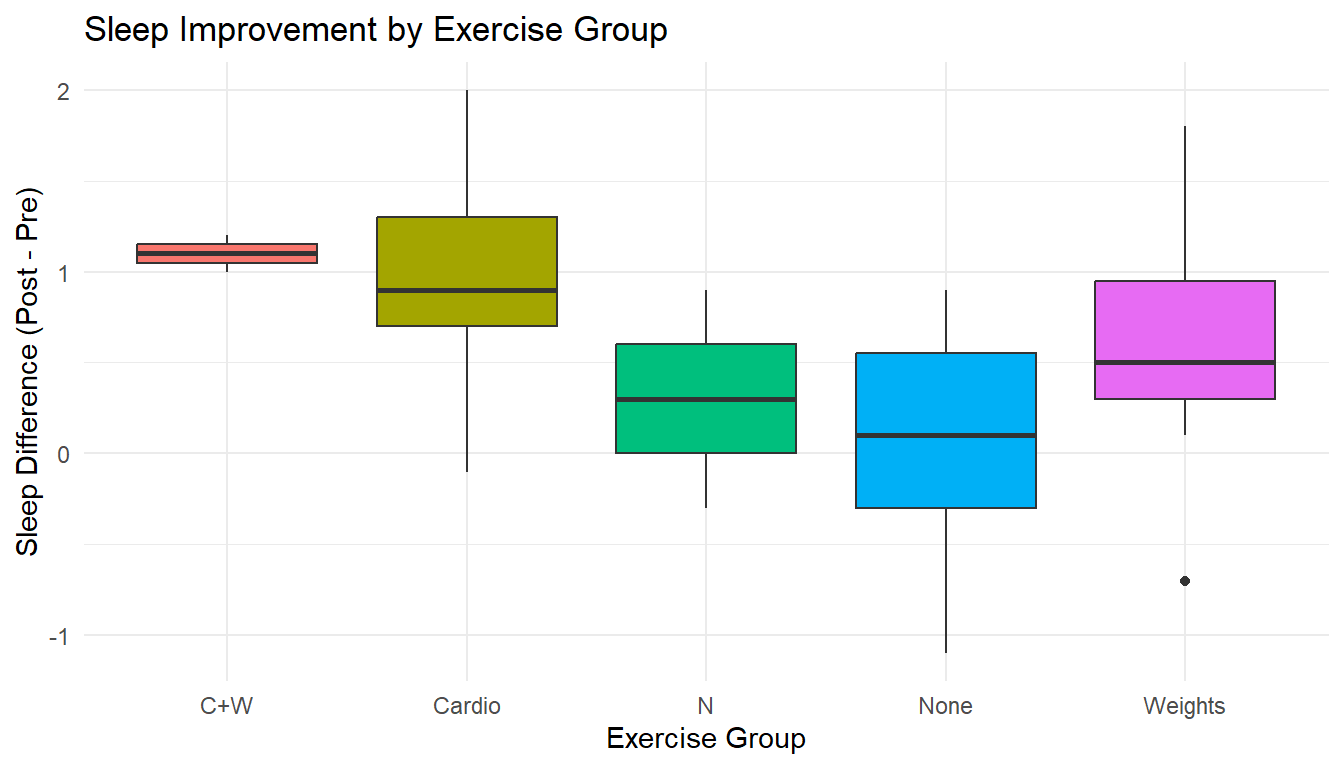

Boxplots of sleep improvement (post–pre) across exercise groups. This visual compares typical improvement and variability by exercise condition.

Figure 4.1: Boxplots of sleep improvement (post–pre) across exercise groups. This visual compares typical improvement and variability by exercise condition.

ggplot(merged_data, aes(x = exercise_group, y = sleep_efficiency, fill = exercise_group)) +
geom_boxplot() +
labs(title = "Sleep Efficiency by Exercise Group",
x = "Exercise Group", y = "Sleep Efficiency (%)") +
theme_minimal() +
theme(legend.position = "none")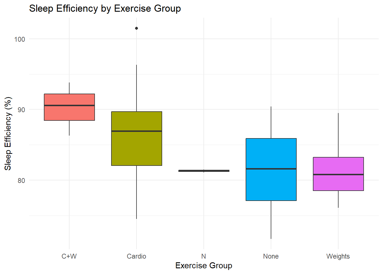

Figure 4.2: Sleep Efficiency by Exercise Group

ggplot(merged_data, aes(x = sleep_difference, y = sleep_efficiency)) +
geom_point(color = "blue") +
geom_smooth(method = "lm", se = FALSE, color = "red") +
labs(title = "Relationship Between Sleep Improvement and Sleep Efficiency",
x = "Sleep Difference (Post - Pre)", y = "Sleep Efficiency (%)") +
theme_minimal()

## `geom_smooth()` using formula = 'y ~ x'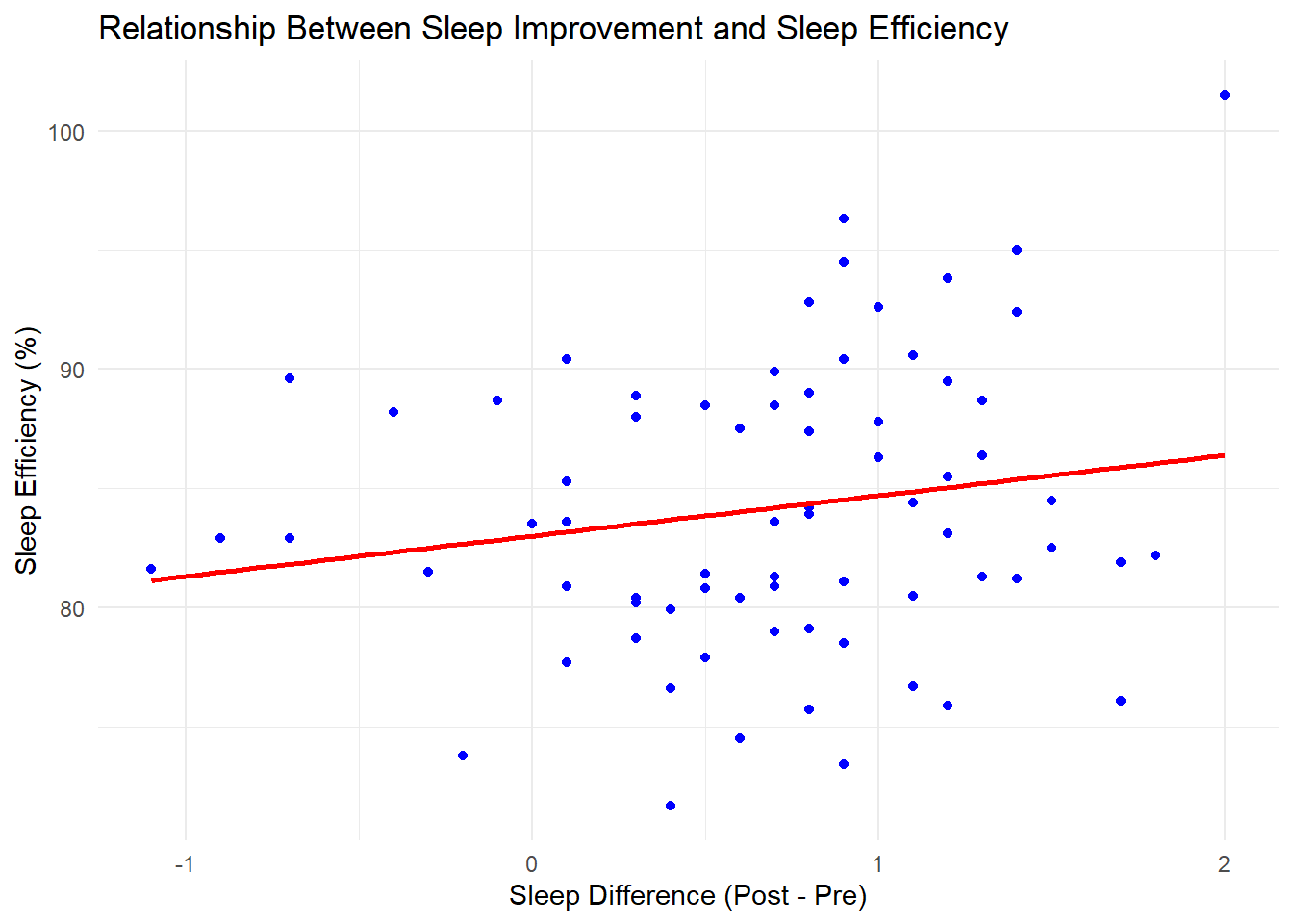

Figure 4.3: Sleep Improvements and Sleep Efficiency

4.5

#Sex

t_sex <- t.test(sleep_difference ~ sex, data = merged_data %>% filter(!is.na(sex)))
t_sex

## 
##  Welch Two Sample t-test
## 
## data:  sleep_difference by sex
## t = 1.3852, df = 64.335, p-value = 0.1708
## alternative hypothesis: true difference in means between group Female and group Male is not equal to 0
## 95 percent confidence interval:
##  -0.09075179  0.50135785
## sample estimates:
## mean in group Female   mean in group Male 
##             0.775000             0.569697

#Age
t_age <- t.test(sleep_difference ~ agegroup2, data = merged_data %>% filter(!is.na(agegroup2)))
t_age

## 
##  Welch Two Sample t-test
## 
## data:  sleep_difference by agegroup2
## t = -1.357, df = 40.85, p-value = 0.1822
## alternative hypothesis: true difference in means between group <40 and group >=40 is not equal to 0
## 95 percent confidence interval:
##  -0.45511702  0.08932755
## sample estimates:
##  mean in group <40 mean in group >=40 
##          0.6421053          0.8250000

Females (M = 0.78, SD = 0.59, n = 40) vs Males (M = 0.57, SD = 0.67, n = 33): p = 0.17. not significant

Age: Younger than 40 (M = 0.64, SD = 0.67, n = 57) vs Age: Forty years or older (M = 0.83, SD = 0.40, n = 16): p = 0.18. not significant

anova_sleep_diff <- aov(sleep_difference ~ exercise_group, data = merged_data)
summary(anova_sleep_diff)

##                Df Sum Sq Mean Sq F value   Pr(>F)    
## exercise_group  4  9.061  2.2653    8.02 2.34e-05 ***
## Residuals      68 19.206  0.2824                     
## ---
## Signif. codes:  0 '***' 0.001 '**' 0.01 '*' 0.05 '.' 0.1 ' ' 1

eta_squared(anova_sleep_diff)

## For one-way between subjects designs, partial eta squared is equivalent
##   to eta squared. Returning eta squared.

## # Effect Size for ANOVA
## 
## Parameter      | Eta2 |       95% CI
## ------------------------------------
## exercise_group | 0.32 | [0.15, 1.00]
## 
## - One-sided CIs: upper bound fixed at [1.00].

tukey_sleep_diff <- TukeyHSD(anova_sleep_diff)
tukey_sleep_diff

##   Tukey multiple comparisons of means
##     95% family-wise confidence level
## 
## Fit: aov(formula = sleep_difference ~ exercise_group, data = merged_data)
## 
## $exercise_group
##                      diff          lwr         upr     p adj
## Cardio-C+W     -0.1294118 -1.026386819  0.76756329 0.9942482
## N-C+W          -0.8000000 -2.159530534  0.55953053 0.4720308
## None-C+W       -1.0133333 -1.955243717 -0.07142295 0.0287638
## Weights-C+W    -0.4894737 -1.414711770  0.43576440 0.5772427
## N-Cardio       -0.6705882 -1.754206665  0.41303019 0.4203454
## None-Cardio    -0.8839216 -1.345549991 -0.42229315 0.0000102
## Weights-Cardio -0.3600619 -0.786642681  0.06651884 0.1375430
## None-N         -0.2133333 -1.334430932  0.90776426 0.9835831
## Weights-N       0.3105263 -0.796600673  1.41765330 0.9338316
## Weights-None    0.5238596  0.009464793  1.03825451 0.0438730

anova_sleep_eff <- aov(sleep_efficiency ~ exercise_group, data = merged_data)
summary(anova_sleep_eff)

##                Df Sum Sq Mean Sq F value  Pr(>F)   
## exercise_group  4  580.7   145.2   4.954 0.00145 **
## Residuals      68 1992.4    29.3                   
## ---
## Signif. codes:  0 '***' 0.001 '**' 0.01 '*' 0.05 '.' 0.1 ' ' 1

eta_squared(anova_sleep_eff)

## For one-way between subjects designs, partial eta squared is equivalent
##   to eta squared. Returning eta squared.

## # Effect Size for ANOVA
## 
## Parameter      | Eta2 |       95% CI
## ------------------------------------
## exercise_group | 0.23 | [0.07, 1.00]
## 
## - One-sided CIs: upper bound fixed at [1.00].

tukey_sleep_eff <- TukeyHSD(anova_sleep_eff)
tukey_sleep_eff

##   Tukey multiple comparisons of means
##     95% family-wise confidence level
## 
## Fit: aov(formula = sleep_efficiency ~ exercise_group, data = merged_data)
## 
## $exercise_group
##                       diff        lwr        upr     p adj
## Cardio-C+W     -3.67745098 -12.813473  5.4585710 0.7912049
## N-C+W          -8.93333333 -22.780654  4.9139870 0.3775963
## None-C+W       -8.86666667 -18.460372  0.7270383 0.0835904
## Weights-C+W    -8.80175439 -18.225646  0.6221370 0.0784124
## N-Cardio       -5.25588235 -16.292936  5.7811713 0.6708789
## None-Cardio    -5.18921569  -9.891072 -0.4873598 0.0232689
## Weights-Cardio -5.12430341  -9.469186 -0.7794209 0.0127670
## None-N          0.06666667 -11.352126 11.4854595 1.0000000
## Weights-N       0.13157895 -11.144918 11.4080760 0.9999997
## Weights-None    0.06491228  -5.174389  5.3042138 0.9999997

4.6

Interpretation:

Sleep Difference ANOVA: F(4,68) = 8.02, p < 0.001, η² = 0.32 - Exercise does significantly improve sleep.

Tukey: “None” < “C+W” and “Cardio”; other differences mostly NS.

Sleep Efficiency ANOVA: F(4,68) = 4.95, p = 0.0015, η² = 0.23 - exercise increases efficiency.

Tukey: No exercise is lower than cardio and weights and just cardio: Weights only was lower than cardio and cardio with weights, also, but not as much as no exercise at all.

Recommendation: Cardio and/or Cardio with weights workouts seem to work best to help improve sleep. People in these groups showed the largest sleep improvements, while those who didn’t exercise had the least sleep improvements. Based on this, cardio only or cardio with weights focused exercise routines are the best way to improve sleep quality, regardless of your age, which did not have significant results. Sex differences did not have significant results either. So if you want to sleep better, hit the gym!

Reflection: This midterm was pretty challenging, mostly because it took me about 12 hours to get everything done. I realized I need to work on managing my time better so I can easily pick up where I left off if I have to take a break. I also want to get a stronger understanding of R code in general so I can work more efficiently. Going forward, I plan to focus on pacing myself and really understanding my code to make future assignments run smoother.