Chapter 6 05-Florida
6.1 Intro
This report analyzes data from Florida counties to see which factors, whether be income, education, or urban environment, best predicts crime rates. The results show that the percentage of urban population is the strongest predictor of crime. Counties with larger urban populations tend to have higher crime rates, while those with higher income and education levels tend to have lower crime, in urban environments. The findings can help us lower crime rates throughout Florida, by pinpointing correlations, and possible causation of crime.
data <- read_excel("C:/Users/laura/OneDrive/Desktop/real_bookdown/Florida County Crime Rates (1).xlsx")


data <- data %>%
  rename(
    County = County,
    Crime = C,
    Income = I,
    HighSchoolGrad = HS,
    UrbanPop = U
  )


data$County <- str_to_title(tolower(data$County))


head(data)
## # A tibble: 6 × 5
## County Crime Income HighSchoolGrad UrbanPop
## <chr> <dbl> <dbl> <dbl> <dbl>
## 1 Alachua 104 22.1 82.7 73.2
## 2 Baker 20 25.8 64.1 21.5
## 3 Bay 64 24.7 74.7 85
## 4 Bradford 50 24.6 65 23.2
## 5 Brevard 64 30.5 82.3 91.9
## 6 Broward 94 30.6 76.8 98.9## County Crime Income HighSchoolGrad
## Length:67 Min. : 0.0 Min. :15.40 Min. :54.50
## Class :character 1st Qu.: 35.5 1st Qu.:21.05 1st Qu.:62.45
## Mode :character Median : 52.0 Median :24.60 Median :69.00
## Mean : 52.4 Mean :24.51 Mean :69.49
## 3rd Qu.: 69.0 3rd Qu.:28.15 3rd Qu.:76.90
## Max. :128.0 Max. :35.60 Max. :84.90
## UrbanPop
## Min. : 0.00
## 1st Qu.:21.60
## Median :44.60
## Mean :49.56
## 3rd Qu.:83.55
## Max. :99.606.2
##                vars  n  mean    sd median trimmed   mad  min   max range  skew
## Crime             1 67 52.40 28.19   52.0   51.60 25.20  0.0 128.0 128.0  0.32
## Income            2 67 24.51  4.68   24.6   24.33  5.34 15.4  35.6  20.2  0.34
## HighSchoolGrad    3 67 69.49  8.86   69.0   69.48 11.56 54.5  84.9  30.4 -0.02
## UrbanPop          4 67 49.56 33.97   44.6   49.75 42.40  0.0  99.6  99.6 -0.02
##                kurtosis   se
## Crime             -0.29 3.44
## Income            -0.70 0.57
## HighSchoolGrad    -1.30 1.08
## UrbanPop -1.49 4.15ggplot(data, aes(x = Income, y = Crime)) +
geom_point() +
geom_smooth(method = "lm", se = TRUE) +
theme_minimal()## `geom_smooth()` using formula = 'y ~ x'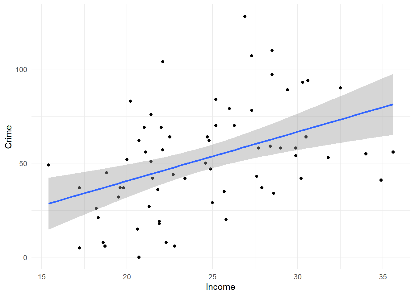
ggplot(data, aes(x = Crime)) +
  geom_histogram(bins = 20, fill = "skyblue", color = "white") +
  theme_minimal()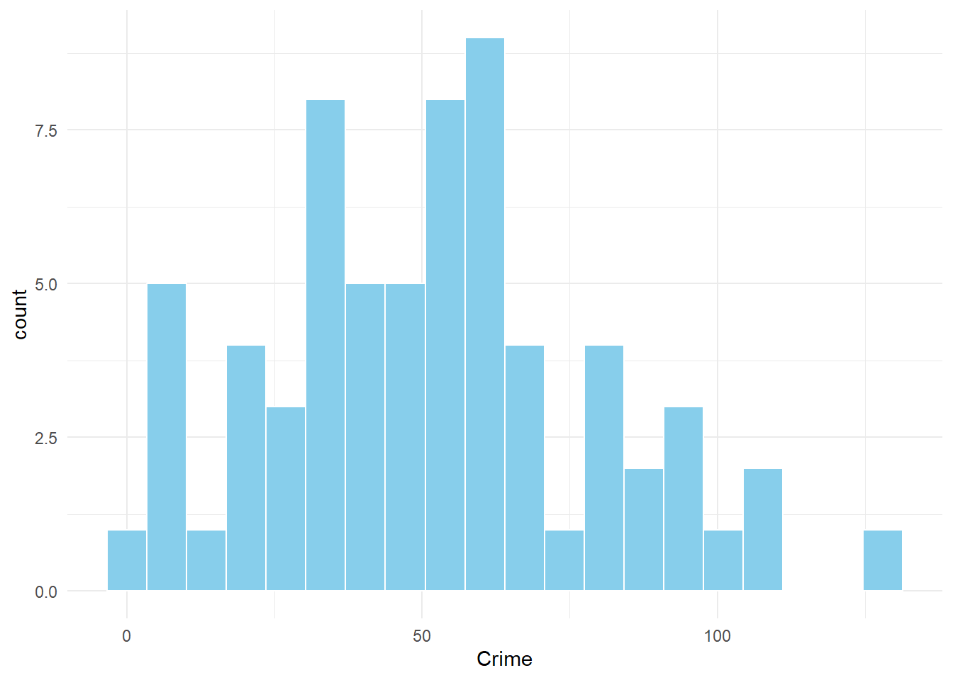
The scatterplot shows a positive relationship (r = .43) between income and crime. As income increases, crime also tends to increase slightly, however, the findings are moderate and with wide variabiltiy between counties. The histogram shows that most Florida counties have moderate crime rates, with a few counties showing higher rates. This distribution shows that crime is consistent across most regions, with urban counties having higher levels of crime.
6.3
##                    Crime    Income HighSchoolGrad  UrbanPop
## Crime          1.0000000 0.4337503      0.4669119 0.6773678
## Income         0.4337503 1.0000000      0.7926215 0.7306983
## HighSchoolGrad 0.4669119 0.7926215      1.0000000 0.7907190
## UrbanPop 0.6773678 0.7306983 0.7907190 1.0000000## Warning: `aes_string()` was deprecated in ggplot2 3.0.0.
## ℹ Please use tidy evaluation idioms with `aes()`.
## ℹ See also `vignette("ggplot2-in-packages")` for more information.
## ℹ The deprecated feature was likely used in the ggcorrplot package.
## Please report the issue at <https://github.com/kassambara/ggcorrplot/issues>.
## This warning is displayed once every 8 hours.
## Call `lifecycle::last_lifecycle_warnings()` to see where this warning was
## generated.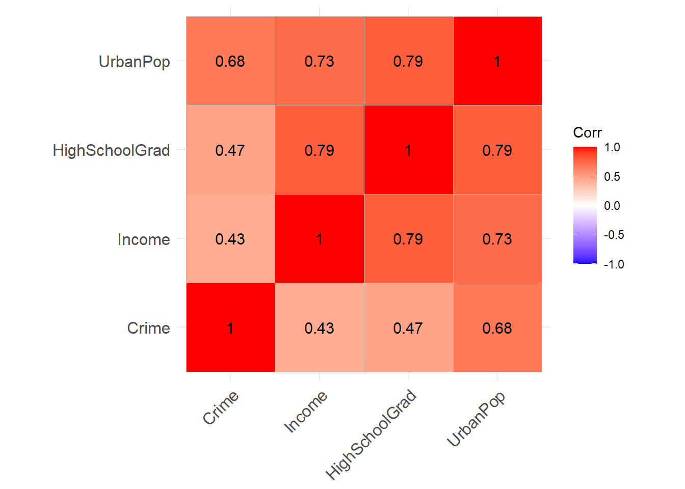
##
## Call:
## lm(formula = Crime ~ Income, data = data)
##
## Residuals:
##     Min      1Q  Median      3Q     Max
## -42.452 -21.347  -3.102  17.580  69.357
##
## Coefficients:
##             Estimate Std. Error t value Pr(>|t|)
## (Intercept) -11.6059    16.7863  -0.691 0.491782
## Income        2.6115     0.6729   3.881 0.000246 ***
## ---
## Signif. codes:  0 '***' 0.001 '**' 0.01 '*' 0.05 '.' 0.1 ' ' 1
##
## Residual standard error: 25.6 on 65 degrees of freedom
## Multiple R-squared:  0.1881, Adjusted R-squared:  0.1756
## F-statistic: 15.06 on 1 and 65 DF, p-value: 0.0002456##
## Call:
## lm(formula = Crime ~ Income + HighSchoolGrad + UrbanPop, data = data)
##
## Residuals:
## Min 1Q Median 3Q Max
## -35.407 -15.080 -6.588 16.178 50.125
##
## Coefficients:
## Estimate Std. Error t value Pr(>|t|)
## (Intercept) 59.7147 28.5895 2.089 0.0408 *
## Income -0.3831 0.9405 -0.407 0.6852
## HighSchoolGrad -0.4673 0.5544 -0.843 0.4025
## UrbanPop 0.6972 0.1291 5.399 1.08e-06 ***
## ---
## Signif. codes: 0 '***' 0.001 '**' 0.01 '*' 0.05 '.' 0.1 ' ' 1
##
## Residual standard error: 20.95 on 63 degrees of freedom
## Multiple R-squared: 0.4728, Adjusted R-squared: 0.4477
## F-statistic: 18.83 on 3 and 63 DF, p-value: 7.823e-09## df AIC
## m1 3 628.6045
## m2 5 603.6764The correlation matrix suggests crime is most strongly associated with urban population. Income and high school graduation also show associations with crime, but these relationships should be interpreted cautiously because they may reflect differences between urban and rural counties (i.e., confounding). In the multiple regression model, urban population remains the strongest predictor after accounting for income and education.
6.4 Memo to the Chief of the Florida Police Department:
Based on my analysis, the multiple regression model best predicts Florida’s county-level crime rates. This model shows that urbanization is the strongest and most significant predictor of crime, meaning that counties with larger urban populations tend to experience higher crime rates. To effectively reduce crime across the state, the Florida Police Department should focus attention and resources on highly urbanized areas, where the risk is greatest.
That said, it would be useful to take a closer look at what types of crimes are most common in these areas before deciding on next steps. If most of the crimes are things like theft, vandalism, or assault, then adding more officers and patrol coverage could help reduce incidents. But if a large portion of the crime comes from social or behavioral issues—like substance abuse, domestic violence, or mental health crises—then it’s just as important to invest in social services, including mental health professionals and social workers. Working together, law enforcement and community services can tackle both the symptoms and the deeper causes of crime. A balanced approach that combines policing with prevention and support will likely be the most effective way to reduce crime in Florida’s urban counties.