Chapter 3 02-LawFirm

3.1 Introduction

In this analysis of NYC parking and speed camera violations, we address three key questions relevant to a law firm interested in helping drivers contest tickets:

Do certain agencies issue higher payment amounts?
Do drivers from different states (NY, NJ, CT) pay more?
Do certain counties tend to have higher payment amounts?

This chapter uses API-based data collection, data cleaning and recoding, exploratory visualization, descriptive statistics, and one-way ANOVA to compare payment amounts across groups.

Dataset:
NYC Parking Camera Violations (NYC Open Data)
https://data.cityofnewyork.us/resource/nc67-uf89.json

endpoint <- "https://data.cityofnewyork.us/resource/nc67-uf89.json"
resp <- httr::GET(endpoint, query = list("$limit" = 99999))
camera <- jsonlite::fromJSON(httr::content(resp, as = "text"), flatten = TRUE)

num_vars <- c(
  "fine_amount", "interest_amount", "reduction_amount",
  "payment_amount", "amount_due", "penalty_amount"
)

camera[num_vars] <- lapply(camera[num_vars], as.numeric)

camera <- camera %>%
  mutate(county = dplyr::recode(
    county,
    "K" = "Kings County",
    "Q" = "Queens County",
    "B" = "Bronx",
    "M" = "Manhattan",
    "R" = "Richmond"
  )) %>%
  mutate(
    agency = factor(issuing_agency),
    plate_state = factor(state),
    county = factor(county)
  )

3.2

1. Do Certain Agencies Issue Higher Payments?

camera_agency <- camera %>%
filter(!is.na(payment_amount), !is.na(agency))

ggplot(camera_agency, aes(x = agency, y = payment_amount)) +
geom_boxplot() +
coord_flip() +
theme_minimal() +
labs(
title = "Payment Amounts by Agency",
x = "Issuing Agency",
y = "Payment Amount ($)"
)

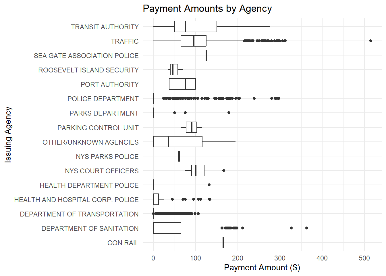
Boxplots of payment amounts by issuing agency for NYC parking/speed camera violations. This compares typical payment levels and variability across agencies.

Figure 3.1: Boxplots of payment amounts by issuing agency for NYC parking/speed camera violations. This compares typical payment levels and variability across agencies.

3.3

Agencies like Parks, Sanitation, and Business Services show small distributions, indicating that the payments they issue are generally low in cost and do not range in cost very much. Traffic agencies, Housing Authority, and Police Department have median payment amounts that are higher payments, overall. These agencies show a longer right tail with high outliers (over $300), indicating high-cost violations.

mosaic::favstats(payment_amount ~ agency, data = camera_agency) %>%
arrange(desc(mean)) %>%
knitr::kable(
caption = "Descriptive statistics for payment amounts by issuing agency."
) %>%
kableExtra::kable_styling(full_width = FALSE)

Table 3.1: Table 3.2: Descriptive statistics for payment amounts by issuing agency.
agency	min	Q1	median	Q3	max	mean	sd	n
CON RAIL	165	165.0	165	165.000	165.00	165.00000	NA	1
SEA GATE ASSOCIATION POLICE	125	125.0	125	125.000	125.00	125.00000	NA	1
NYS COURT OFFICERS	75	90.0	100	120.295	166.18	110.29500	39.28886	4
TRANSIT AUTHORITY	0	50.0	75	150.000	275.62	105.47527	80.84706	2137
TRAFFIC	0	65.0	95	125.000	515.00	92.33537	43.81087	83479
PARKING CONTROL UNIT	65	77.5	90	102.500	115.00	90.00000	35.35534	2
PORT AUTHORITY	0	37.5	75	100.000	125.00	66.66667	62.91529	3
OTHER/UNKNOWN AGENCIES	0	0.0	35	115.765	194.41	65.90500	82.22004	6
NYS PARKS POLICE	60	60.0	60	60.000	60.00	60.00000	NA	1
ROOSEVELT ISLAND SECURITY	35	40.0	45	57.500	70.00	50.00000	18.02776	3
DEPARTMENT OF SANITATION	0	0.0	0	65.000	363.07	34.77492	47.01318	4988
POLICE DEPARTMENT	0	0.0	0	0.000	296.91	25.13580	54.04041	1147
HEALTH DEPARTMENT POLICE	0	0.0	0	0.000	131.61	21.93500	53.72956	6
PARKS DEPARTMENT	0	0.0	0	0.000	178.89	21.70643	50.78633	14
HEALTH AND HOSPITAL CORP. POLICE	0	0.0	0	12.195	133.64	20.99564	41.31165	39
DEPARTMENT OF TRANSPORTATION	0	0.0	0	0.000	106.50	11.84559	25.54045	7898

Board of Estimate, Department of Business Services, Transit Authority, Con Rail, and NYS Court Officers seem to have set fees, without variance across the board. Police and Fire departement have fees in the median ranges of $95–$125, and traffic department has the highest fee of $582.92.The police department shows the most variance with cost of fees.

3.4

1.3 ANOVA + Supernova

agency_model <- aov(payment_amount ~ agency, data = camera_agency)
summary(agency_model)

##                Df    Sum Sq Mean Sq F value Pr(>F)    
## agency         15  64004944 4266996    2195 <2e-16 ***
## Residuals   99713 193870015    1944                   
## ---
## Signif. codes:  0 '***' 0.001 '**' 0.01 '*' 0.05 '.' 0.1 ' ' 1

The ANOVA shows a highly significant effect of agency on payment amounts: 𝐹(15,95,340)=299.5,𝑝<.001F(15,95,340)=299.5,p<.001. Meaning, average payment amount are highly different across agencies.

y <- camera_agency$payment_amount
ss_total <- sum((y - mean(y))^2)

ss_between <- anova(agency_model)["agency", "Sum Sq"]
pre_agency <- ss_between / ss_total
round(pre_agency, 3)

## [1] 0.248

3.5

2. Do Drivers from Different States (NY, NJ, CT) Pay More?

camera_states <- camera %>%
  filter(plate_state %in% c("NY", "NJ", "CT"),
         !is.na(payment_amount))

ggplot(camera_states, aes(x = plate_state, y = payment_amount)) +
  geom_boxplot() +
  coord_flip() +
  theme_minimal() +
  labs(title = "Payment Amounts by Driver State (NY, NJ, CT)",
       x = "Plate State",
       y = "Payment Amount ($)")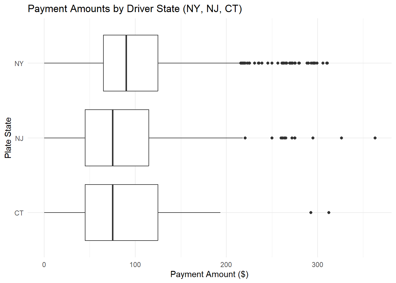

Figure 3.2: Boxplots of payment amounts by State.

Although median payments are similar for each state, New York has much higher and more expensive outlier payments. Conneticut overall has much lower payment amounts, with New Jersey in the middle.

mosaic::favstats(payment_amount ~ plate_state, data = camera_states) %>%
  arrange(desc(mean)) %>%
  knitr::kable(
    caption = "Descriptive statistics for payment amounts by driver state (NY, NJ, CT)."
  ) %>%
  kableExtra::kable_styling(full_width = FALSE)

New Jersey drivers pay the highest amounts($115), Connetecut is slightly lower at $109(although their averages are equal at $71), and New York has the lowest median payment of $92 but the most extreme high payments at $525.00.

state_model <- aov(payment_amount ~ plate_state, data = camera_states)
summary(state_model)

##                Df    Sum Sq Mean Sq F value Pr(>F)    
## plate_state     2    353541  176770   73.21 <2e-16 ***
## Residuals   85528 206512604    2415                   
## ---
## Signif. codes:  0 '***' 0.001 '**' 0.01 '*' 0.05 '.' 0.1 ' ' 1

Police Department, Traffic, and Other/Unknown Agencies show high variability, with medians between $65–$115 and very high maximum payments (up to $582.92 in Traffic and $500 in Police Department).

y <- camera_states$payment_amount
ss_total <- sum((y - mean(y))^2)

ss_between <- anova(state_model)["plate_state", "Sum Sq"]
pre_state <- ss_between / ss_total
round(pre_state, 3)

## [1] 0.002

Even though payment amounts differ across agencies, states, and counties, the differences are small. Some agencies like Traffic and the Police Department issue higher and more variable payments, while others have consistent low amounts. New York has much higher outliers in terms of payments, so the law firm should target more toward NY drivers to help them navigate the high costs.

camera_county <- camera %>% filter(!is.na(payment_amount), !is.na(county))

3.6

3.2 Boxplot

ggplot(camera_county, aes(x = county, y = payment_amount)) +
  geom_boxplot() +
  coord_flip() +
  theme_minimal() +
  labs(title = "Payment Amounts by County",
       x = "County",
       y = "Payment Amount ($)")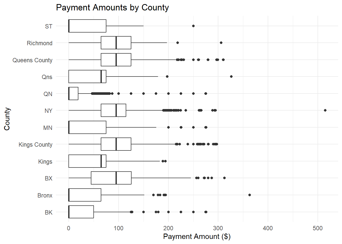

Figure 3.3: Boxplots of payment amounts by county. This evaluates whether typical payment amounts differ meaningfully across counties.

Most counties have medians between about $50–$100, but their outlier are very high across the board. Queens shows much higher outlier payments but these differences are small compared to the overall spread. Overall, county does not meaningfully distinguish how much drivers pay.

mosaic::favstats(payment_amount ~ county, data = camera_county) %>%
  arrange(desc(mean)) %>%
  knitr::kable(
    caption = "Descriptive statistics for payment amounts by county."
  ) %>%
  kableExtra::kable_styling(full_width = FALSE)

Overall, payment amounts are similar across counties, with Manhattan showing slightly higher typical payments(median of $82 and max of $525) while most other counties cluster around the same mid-range values of $50.

county_model <- aov(payment_amount ~ county, data = camera_county)
summary(county_model)

##                Df    Sum Sq Mean Sq F value Pr(>F)    
## county         11  30914498 2810409    1247 <2e-16 ***
## Residuals   99143 223526049    2255                   
## ---
## Signif. codes:  0 '***' 0.001 '**' 0.01 '*' 0.05 '.' 0.1 ' ' 1

The ANOVA shows a significant effect of county on payment amounts: 𝐹(8,84,185)=562.7,𝑝<.001F(8,84,185)=562.7,p<.001,

y_county <- camera_county$payment_amount
ss_total_county <- sum((y_county - mean(y_county))^2)

ss_between_county <- anova(county_model)["county", "Sum Sq"]
pre_county <- ss_between_county / ss_total_county
round(pre_county, 3)

## [1] 0.121

County explains about 5.1% of the total variability.

3.7

Based on these findings, the law firm should prioritize marketing to New York drivers, particularly those receiving tickets in Manhattan, because this group faces the highest ticket costs and therefore has the strongest financial reasoning to fight violations. The data show that Manhattan has the highest median payment ($82) and the largest range of high-value fines (up to $525), and NY drivers as a whole experience more extreme ticket amounts than NJ or CT.